External multiplicity-based triggers (muon veto)¶

This tutorial shows how to use the functions in reboost.pmts to apply a multiplicity-based trigger scheme similar to the LEGEND muon veto. This is especially useful for external veto systems with an independent DAQ or trigger system that is detached from the main detector system. The hit building in this tutorial is independent from the main reboost hit building or TCM handling, but the resulting veto information can still be applied to the main detector processing chain.

Two workflows are shown below. The first processes the veto data without using the TCM and therefore only reconstructs the response of the external veto system. The second uses the TCM built by reboost to apply the veto response to hits in the main detectors.

The example uses the LEGEND-200 muon veto, but the same logic can be used for any multiplicity-based trigger system.

Isolated event building¶

Reading the data¶

Isolated event building only requires the input stp file from remage. For the LEGEND muon veto we are only interested in the PMT detectors, so we iterate over all detectors and keep the ones whose name contains pmt. The same filter can also be used to exclude detectors, for example broken PMTs.

import awkward as ak
import numpy as np
import lh5

stp_file = "..."  # (adjust this)
stps = lh5.read("stp", stp_file)

records = []
lengths = []
for det, table in stps.items():
    if "pmt" not in det.lower():
        continue

    ak_table = table.view_as("ak", with_units=True)
    if ak_table.time.ndim == 2:
        evtid, time = ak.broadcast_arrays(ak_table.evtid, ak_table.time)
        time = ak.with_parameter(
            ak.flatten(ak_table.time),
            "units",
            ak.parameters(ak_table.time)["units"],
        )
        flat_table = ak.zip(
            {
                "evtid": ak.flatten(evtid),
                "time": time,
            }
        )
    else:
        flat_table = ak_table

    records.append(flat_table)
    lengths.append(len(flat_table))

# Concatenating and unflattening is faster than creating ak.Array(records) directly.
flat = ak.concatenate(records)
input_arr = ak.unflatten(flat, lengths)

The processing further down the line expects flat input arrays. If remage was run without flat_output=True, the data therefore has to be flattened again. This is the reason for the if block above. In that case remage groups timestamps according to the TCM, but for this part we do not want the TCM grouping, so we undo it.

It is also recommended to use the remage macro option /RMG/Output/NtupleUseVolumeName true so the detector names can be filtered directly instead of having to rely on the uid.

We can now inspect the input shape. For the LEGEND-200 muon veto, with all 53 installed PMTs, the expected type looks like this:

print(f"Input type: {ak.type(input_arr)}")

Input type: 53 * var * {evtid: int64, time: float64[parameters={"units": "ns"}]}

The first axis corresponds to the number of detectors, and the second axis contains the flattened entries/hits. Because the number of entries can vary per detector, this is a jagged array.

Aligning the data¶

Next we regroup the hits by event id. The data also has to be padded so that all detectors have their event \(n\) at the same position, even if a detector has no entries for this or previous events. For this we use reboost.pmts.align_detectors.

from reboost.pmts.functions import align_detectors

re_shaped_arr, unique_evtids = align_detectors(
    input_arr,
    field="time",
    return_event_ids=True,
)

print(f"re_shaped_arr: {ak.type(re_shaped_arr)}")
print(f"Unique event IDs: {ak.type(unique_evtids)}")

re_shaped_arr: 53 * [791 * var * float64[parameters={"units": "ns"}], parameters={"units": "ns"}]
Unique event IDs: 791 * int64

This function adds a new dimension corresponding to one Geant4 event. In this example there are 791 unique events in the dataset. If return_event_ids=True, the function also returns the unique event ids, which would otherwise be lost. unique_evtids[2] returns the event id of re_shaped_arr[:, 2, :], so it is an important mapping back to the original event.

Because of the padding required to align the events properly, this array can consume a lot of RAM. It is typically the most memory-intensive object in this processing chain.

Applying the trigger scheme¶

The next step is to apply the actual trigger logic. reboost.pmts.build_hardware_triggers supports two trigger modes. The simplest mode is defined by a single multiplicity_threshold. In that case a global search is performed over all detectors for every event. The other important parameters are timegate and trigger_deadtime. A trigger is created for every timegate-sized window in which the multiplicity threshold is reached. The trigger is assigned the time of the photon that caused the threshold to be reached. In a second step, all trigger times within trigger_deadtime after a previous trigger are discarded.

The second trigger mode lets you split the detectors into zones. Each zone can have its own multiplicity threshold, which is derived only from detectors in that zone. The resulting trigger is still global, so information about which zone caused the trigger is not retained, and the trigger deadtime is also applied globally. To use this mode, pass a dictionary with detector indices for each zone. The example below uses three trigger zones for LEGEND-200. Since the detector names are sorted after reading, these zones can be defined with simple index ranges. If you remove detectors, these ranges need to be updated accordingly. This is the slowest part of the processing, except for the optional trace building.

from reboost.pmts.functions import build_hardware_triggers

channels_pill = list(range(0, 10))  # detectors 0-9 are pillbox PMTs
channels_floor = list(range(10, 30))  # detectors 10-30 are floor PMTs
channels_wall = list(range(30, 53))  # detectors 30-52 are wall PMTs

det_groups_dict = {
    "pillbox": {
        "detector_indices": channels_pill,
        "threshold": 6,
    },  # Threshold 6 in the pillbox
    "floor": {
        "detector_indices": channels_floor,
        "threshold": 4,
    },  # Threshold 4 for wall/floor
    "wall": {"detector_indices": channels_wall, "threshold": 4},
}

triggers = build_hardware_triggers(
    re_shaped_arr,
    trigger_groups=det_groups_dict,
    timegate=60,
    trigger_deadtime=880,
)

print(f"triggers: {ak.type(triggers)}")

triggers: 53 * [791 * var * float64, parameters={"units": "ns"}]

The first detector axis is only kept for compatibility with the reboost processor rules. Because the triggers are applied globally, every row in the 53 detector rows in this example contains the same elements. The third variable dimension represents the possibility of multiple triggers per Geant4 event. ak.num(triggers[0], axis=2) returns the number of triggers for each event. triggers[0][4][1] returns the timestamp of the second trigger of the fifth event. If that entry does not exist, the call raises an error.

Hit building¶

While the trigger array is already useful on its own, its main purpose is to build hits. To build hits, you need to provide trace_length, time_per_sample, and trigger_position. To better understand the output, it can be helpful to first inspect the optional build_traces function. build_traces reconstructs a full detector trace from the arguments above. This is computationally expensive, so it is best used for a few selected events rather than the full dataset.

from reboost.pmts.functions import build_traces

triggers = triggers[0]  # remove the decorative axis
trace = build_traces(
    re_shaped_arr[:, :10],
    triggers[:10],
    trace_length=220,
    time_per_sample=4,
    trigger_position=110,
)

print(ak.type(trace))

53 * 10 * var * 220 * int16

We can now plot a single event by looping over the detectors. With 53 detectors, a meaningful legend would be unwieldy, so the plot is shown without one.

import matplotlib.pyplot as plt

plt.figure(figsize=(10, 5))
for i in range(len(trace)):
    plt.plot(trace[i, 0, 0])

plt.title("Traces for Event 1, Trigger 1", fontsize=16)
plt.xlabel("Sample Index", fontsize=14)
plt.ylabel("Amplitude in p.e.", fontsize=14)
plt.tick_params(axis="both", which="major", labelsize=12)
plt.tight_layout()

png

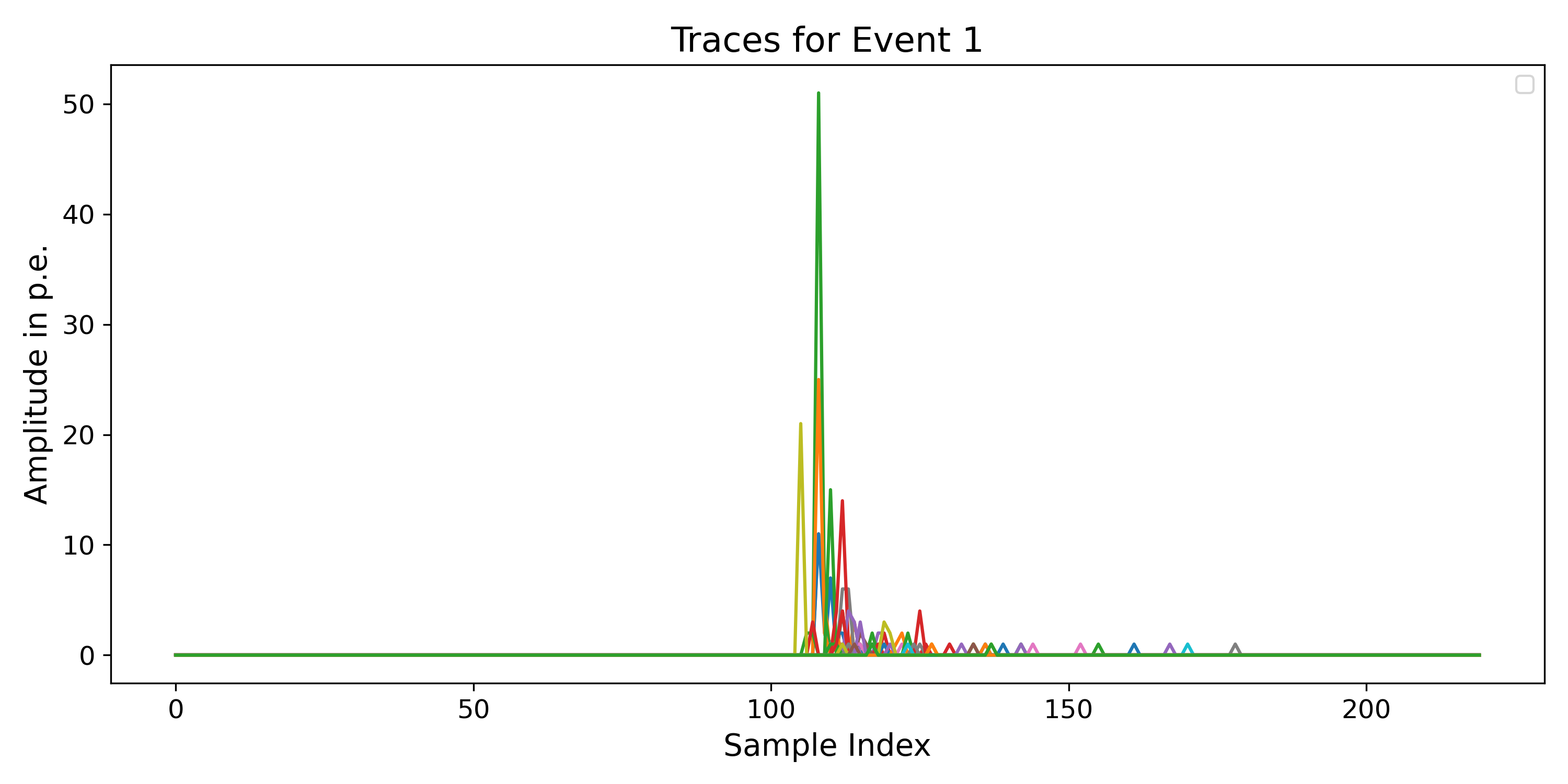
This is what an idealized PMT waveform looks like after deconvolution from the electronic response. In practice, we do not have idealized waveforms, so there are many ways to reconstruct the number of photoelectrons from a detector waveform. The best solutions usually approximate the pulse height in some form. To mimic that, build_hits takes the maximum of the waveform for each detector. In practice, build_hits does not need to build the full waveform to find the maximum sample, so it is much faster. Note that the result is strongly influenced by time_per_sample, so this value should match the detector time resolution.

Now, after this optional detour, we can look at the output of build_hits. It returns the reconstructed number of photoelectrons seen by each detector for each hardware trigger.

from reboost.pmts.functions import build_hits

hits = build_hits(
    re_shaped_arr,
    triggers,
    trace_length=220,
    time_per_sample=4,
    trigger_position=110,
)

hits: 53 * 791 * var * int32

Event building¶

To get a typical muon veto integral light versus multiplicity plot, we now only need to calculate those two values.

integral_light = ak.sum(hits, axis=0)
multiplicity = ak.sum(hits > 0, axis=0)

print(f"integral_light: {ak.type(integral_light)}")
print(f"multiplicity: {ak.type(multiplicity)}")

integral_light: 791 * var * int64
multiplicity: 791 * var * int64

For simplicity, we flatten the second trigger axis into the first event axis to make a 2D plot:

integral_light_flat = ak.to_numpy(ak.flatten(integral_light))
multiplicity_flat = ak.to_numpy(ak.flatten(multiplicity))

xlims = (0, 54)
ylims = (1, 10000)
y_bins = np.logspace(np.log10(ylims[0]), np.log10(ylims[1]), 100)
x_bins = min(xlims[1] - xlims[0], 100)

plt.figure(figsize=(10, 5))
plt.hist2d(
    multiplicity_flat,
    integral_light_flat,
    bins=(x_bins, y_bins),
    range=[xlims, ylims],
    cmap="viridis",
    norm=mpl.colors.LogNorm(),
)
plt.colorbar(label="Counts")
plt.title("Integral Light vs Multiplicity", fontsize=16)
plt.xlabel("Multiplicity", fontsize=14)
plt.yscale("log")
plt.ylabel("Integral Light (p.e.)", fontsize=14)
plt.tick_params(axis="both", which="major", labelsize=12)
plt.tight_layout()

png

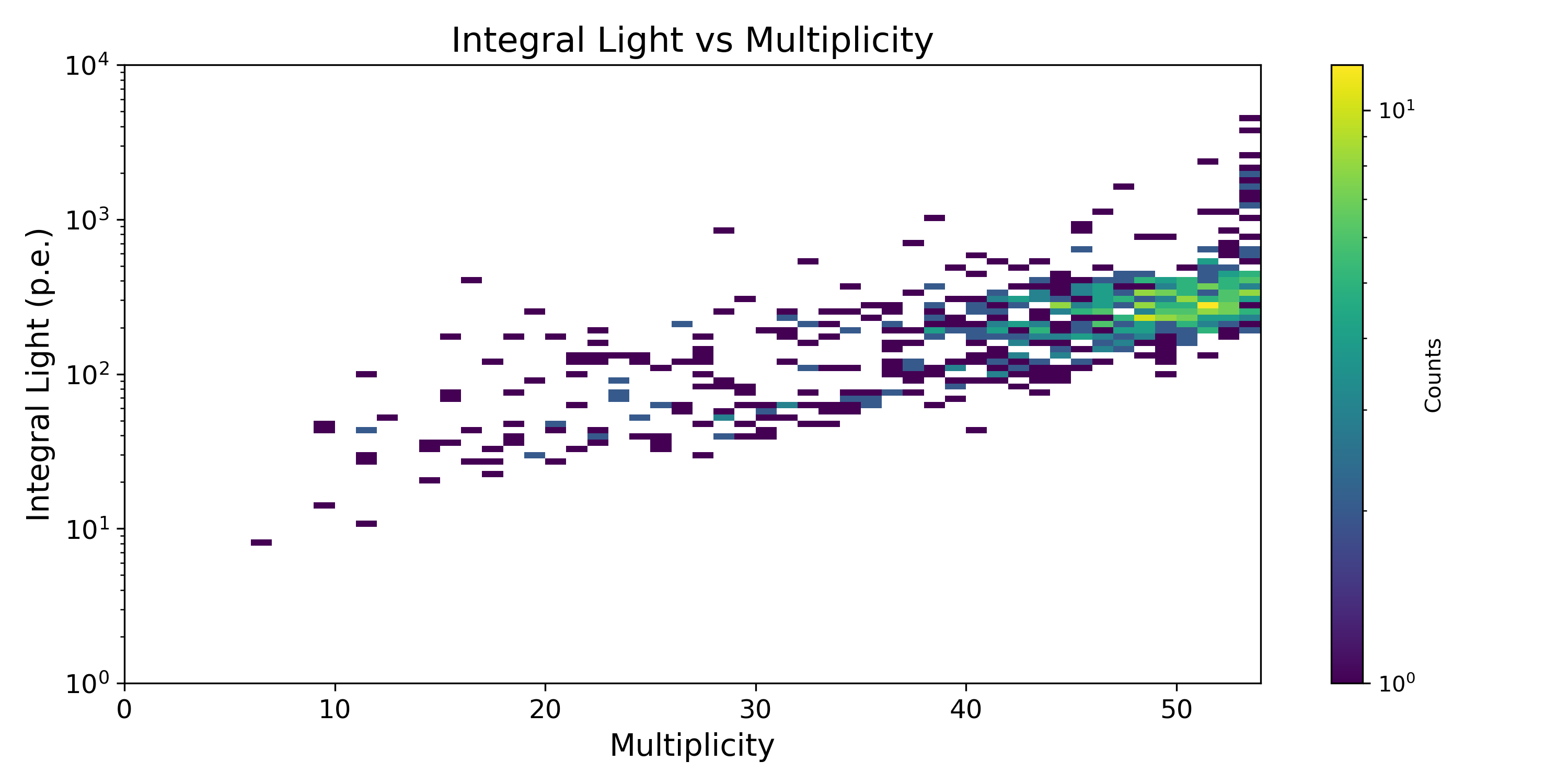
Even with relatively low statistics, this already looks like the familiar muon veto plot and should converge to it with more events. The unique_evtids array can now be used to apply this veto system to other detectors in the same event. It gives the Geant4 event id for each row in multiplicity, integral_light, and triggers. The triggers array stores the trigger timestamp, and the other two arrays can be used to apply multiplicity or integral-light cuts.

Using the TCM, WIP¶

You can also use the TCM to read in the data instead. This requires the read_hits function, which currently only exists as a helper function in legend-simflow, but is planned to move to reboost. This section will be updated once that function is implemented.

from reboost.pmts.functions import group_by_detector

re_shaped_arr = group_by_detector(times, tcm_ak["stp"].table_key, usable_pmts)
print(ak.type(re_shaped_arr))

53 * 824 * var * float64

The group_by_detector() function performs the same job as align_detectors(), so the result should be equivalent. The difference is that the input data comes from the TCM instead of the Geant4 event grouping. In this example we get 824 events instead of 791. The stp data itself does not change, but the basic remage TCM grouping can split one Geant4 event into multiple time-coincidence events. This can be avoided by specifying an unrealistically large grouping time, but at that point the TCM no longer adds much value.

The first argument of group_by_detector() is the result of the aforementioned read_hits function. The second argument is the table_key field of the TCM. The third required argument, usable_pmts, is a list of detector UIDs that should be considered. The first axis of the result array is ordered according to usable_pmts, so the 53 detectors will appear in that order. By contrast, align_detectors() preserves the input ordering. The reason for this difference is that the input times array has a completely different shape from the resulting re_shaped_arr.

After this, the rest of the processing chain should be exactly the same. The resulting plot should also be the same after flattening, as long as the time windows used for the processing functions are smaller than the TCM grouping time. The number of rows and triggers per row will still differ, because the TCM may split one event into two rows. This needs to be taken into account when applying a veto that is longer than the chosen TCM grouping time.